
Sergey - stock.adobe.com
Common ML patterns: Central tendency and variability
Four common patterns provide approaches to solving machine-learning problems. Learn how two -- central tendency computation and variability computation -- work.
This article is excerpted from the course "Fundamental Machine Learning," part of the Machine Learning Specialist certification program from Arcitura Education. It is the fourth part of the 13-part series, "Using machine learning algorithms, practices and patterns."
Let's focus on a collection of machine learning techniques documented as "patterns." A pattern provides a proven solution to a common problem individually documented in a consistent format; usually, it is part of a larger collection.
Each pattern is documented in a profile comprised of the following parts:
- Requirement. Every pattern description begins with a requirement. A requirement is a concise single sentence, in the form of a question, that asks what the pattern addresses.
- Problem. The issue causing a problem and the effects of the problem are described in this section, which may be accompanied by a figure that further illustrates the "problem state." It is this problem for which the pattern is expected to provide a solution.
- Solution. The solution explains how the pattern will solve the problem and fulfill the requirement. Often the solution is a short statement that may be followed by a diagram that concisely communicates the final solution state. "How-to" details are not provided in this section but are instead located in the Application section.
- Application. This section describes how the pattern can be applied. It can include guidelines, implementation details, and even a suggested process.
Explore two patterns: The central tendency and the variability computations
Let's look at two of four common patterns that document data-exploration techniques, which act as a common entry point for machine learning problem-solving tasks: the central tendency computation and variability computation.
Central tendency computation: Overview
- Requirement: How can the makeup of a data set be determined in terms of the normal set of values?
- Problem: Before solving a machine learning problem, a preliminary understanding of the input data is required. However, not knowing which techniques to start with can negatively impact the subsequent model development.
- Solution: The data set is analyzed and the values that normally occur around the center of a distribution, plus the most occurring values, are calculated via established statistical techniques.
- Application: The data set is arranged in ascending or descending order, and the measures of central tendency (mean, median, and mode) are calculated.
Central tendency computation: Explained
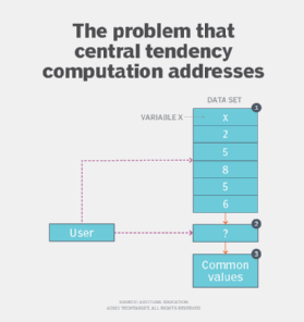
Problem
Before a model can be trained, it is imperative to fully understand the nature of the data set at hand. Failure to do so may lead to wrong assumptions or the use of the wrong type of algorithm. At a very basic level, to develop an understanding of the data set it is important to know which value or values normally appear in the data set. However, with a plethora of quantitative and qualitative techniques at hand, applying the most suitable analysis technique can be a daunting task. In Figure 1, X is a variable in a data set. To determine its value, a technique needs to be applied to obtain the common set of values (2) and (3).
Solution
The guiding data analysis principle dictates that the best way to determine a commonly occurring set of values is to capture the average behavior of the data set by finding out which values, or range of values, appear most frequently. In a distribution, such values are normally found towards the center. However, in cases involving a few extreme set of values, this center is pulled to one side. This results in a false center, in which case a count of the values that occur the most provides a more robust average behavior of the data set.
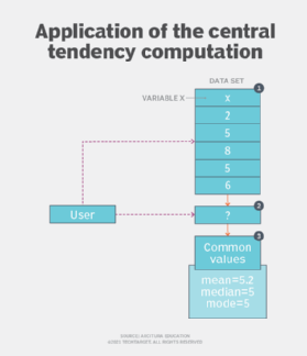
Application
To obtain the average behavior of the data set, the measures of central tendency that include mean, median, and mode are calculated (Figure 2). These three measures are also commonly referred to as averages. These averages help us to summarize data, compare two sets of values (distributions) and compare a single value against the rest of the values in the distribution.
In most cases, calculating the mean (also commonly referred to as the average) provides a good measure for getting an idea of which value of a variable is the most common. For example, the mean height of a group of individuals can be taken to determine what the average height is. Mean is calculated by taking the sum of all values and dividing it by the number of values. However, mean is generally used when the values do not change much and increase or decrease in a normal manner.
Mean is affected by the presence of outliers. When outliers occur, finding the median or mode is recommended as they remain robust despite outliers. For example, with a set of values for household income where most of the values occur towards the center of the distribution but a few large values occur on the right side (high income), finding the average income via the mean would provide an incorrect value. That is, the few abnormally high values will skew the mean. Calculating the median or mode, however, provides an accurate measure as these measures do not consider the entire set of values in a distribution for calculation purposes.
Median is calculated by arranging the set of values in ascending order and then finding the middle value, whereas mode is simply the most frequently occurring value in the distribution. A distribution can have two or more modes, in which case the distribution is bimodal or multimodal, respectively. (See Figure 2.)
Variability computation: Overview
- Requirement: How can the spread of values for a single variable in a data set be determined?
- Problem: Developing an intuition about a data set involves determining the behavior of uncommon values of data. Failure to do so may result in treating abnormal values as normal.
- Solution: The behavior of the uncommon values in a data set is expressed in the form of the spread of values and is quantified via the application of proven statistical techniques.
- Application: The numerical values in the data set are identified and measures of variation -- including range, interquartile range (IQR), variance and standard deviation -- are calculated.
Variability computation explained
Problem
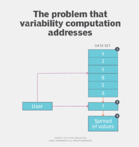
The application of the central tendency computation pattern enables a preliminary understanding about the makeup of a distribution in terms of finding the central value. However, its application alone fails to address the requirement of determining the behavior of non-central values. This is an important aspect of exploratory analysis prior to model development, since finding out which values, apart from the central one, normally appear in a distribution is helpful when building an effective model. (See Figure 3.)
Solution
The spread of values from the central value (mean, median or mode) is quantified to find out how tightly or loosely packed the values of a distribution are. The spread can either be defined in terms of the extremities of the distribution or the variation in values.
Application
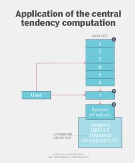
The application of this pattern requires the calculation of measures of variation, including range, interquartile range (IQR), variance and standard deviation. (See Figure 4.)
The range is a statistic obtained by subtracting the minimum value from the maximum value that indicates the spread or width of data. The range is heavily affected by the presence of extreme values, as the presence of a single extreme value gives the impression that the values are spread over a very large range. The averages (mean, median and mode) provide central value, while range provides insight to the variation in the data. Using range, two different sets of values can be compared in terms of variation in their values.
Quartiles represent three values that divide the data into four equal portions, obtained by first arranging the data values in ascending order and then dividing the data into four quarters. The first, second and third quartiles are known as lower quartile (Q1), median (Q2) and upper quartile (Q3).
Q1, Q2 or Q3 represent values below which 25%, 50% or 75% of data values exist, respectively. Based on quartiles, the IQR is calculated. The IQR is the set of values between Q1 and Q3. That is, IQR = Q3 – Q1. IQR provides a simple method of eliminating outliers from a data set as outliers normally occur outside of Q1 and Q3.
The variance is a non-negative value that shows how spread the values are compared to the mean of the values or center of a distribution. A small variance shows that there is a comparatively small difference between the values and the mean value, and that the values occur close to each other in a distribution. A large variance shows that there is comparatively large difference between the values and the mean value, and that the values occur far from each other.
The standard deviation is another non-negative value to view the spread of the values from the center of the distribution and is simply the square root of the variance. The calculated value is known as one standard deviation, and it is expressed in the same units as the values in the distribution.
The standard deviation is generally more useful than a variance for descriptive purposes, whereas a variance is generally more useful mathematically. The lower the variance and standard deviation, the less spread out and the closer to the mean value the values are. The variance and standard deviation enable us to measure how consistently a process generates data, for example to analyze which bottle-filling machine fills bottles on a more consistent basis.
In the next article in this series, we'll look at the remaining two data-exploration patterns: associativity computation and the graphical summary computation.
View the full series
This lesson is one in a 13-part series on using machine learning algorithms, practices and patterns. Click the titles below to read the other available lessons.
Course overviewLesson 1: Introduction to using machine learning
Lesson 2: The supervised approach to machine learning
Lesson 3: Unsupervised machine learning: Dealing with unknown data
Lesson 4
Lesson 5: Associativity, graphical summary computations aid ML insights
Lesson 6: How feature selection, extraction improve ML predictions
Lesson 7: 2 data-wrangling techniques for better machine learning
Lesson 8: Wrangling data with feature discretization, standardization
Lesson 9: 2 supervised learning techniques that aid value predictions
Lesson 10: Discover 2 unsupervised techniques that help categorize data
Lesson 11: ML model optimization with ensemble learning, retraining
Lesson 12: 3 ways to evaluate and improve machine learning models
Lesson 13: Model optimization methods to cut latency, adapt to new data